Key features of scope2d
- General GUI
- Instances
- Markers
- Charters
- Plot Scales
- Calculators
- Curve Fitters
- scope2d Generic CSV File Format
General GUI Top
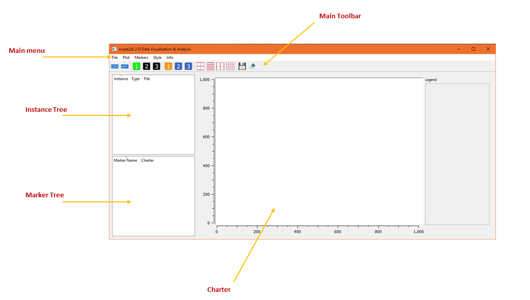
scope2d has 5 main GUI sections.
-
Instance Tree: The tree that displays currently loaded instances. You can interact with loaded instances by right clicking them on the instance tree and selecting one of the available operations.
-
Marker Tree: The tree that displays existing markers. You can interact with markers by right clicking them on the marker tree and selecting one of the available operations.
-
Charter: The canvas on which the plots and markers are drawn.
-
Main Menu: Main menu of the program.
-
Main Toolbar: Toolbar for quickly accessing the operations that are frequently used.
Instances Top
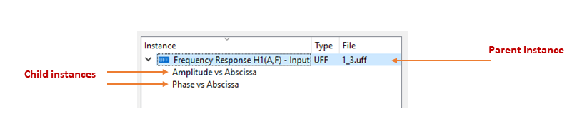
scope2d uses instances to work with data. Instances contain the data and the plot to be visualized and analyzed and any interaction with these data are made through instances.
There are two types of instances; parent instances and child instances. Parent instances contain the raw data; child instances contain the plots. So the data are interacted with through parent instances, while the plots are interacted with through child instances.
Making plots Top
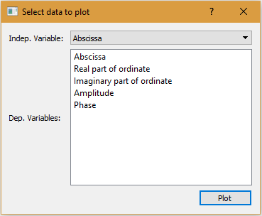
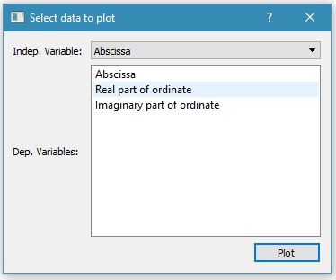
To make plots, right click a parent instance and select “Make plots”. Make plots dialog will pop up and it will be possible to select multiple dependent variables to plot against the same independent variable. It is possible to make plots of different independent plots on the same charter.
Deleting data columns Top
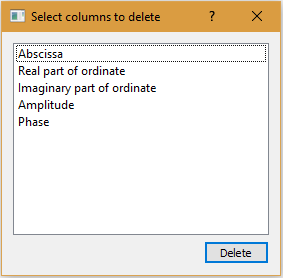
Parent instances contain data as columns. It is possible to delete columns of data that a parent instance contains by simply right clicking the parent instance and selecting “Delete columns”. A dialog will open and it is possible to select a single or multiple columns to delete. Any plot related to the data to be deleted are automatically deleted, so it is not needed to delete plots manually before deleting data columns.
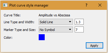
Plot style management Top
Plot style controls are available through child instances. Simply select and right click a single or multiple child instances and select “Manage style”, which will pop up a style management dialog. If multiple child instances are selected, the resulting style will be applied to all of them.
Markers Top
Markers are useful for data analysis in scope2d. Markers can be used for a variety of tasks such as finding important frequency components in the frequency spectrum of a signal or finding repetitions or other important events in a time signal.
There are 4 kinds of markers available in scope2d:
- Vertical
- Horizontal
- Cross
- Point
To draw a marker, go to “Markers” menu on the main menubar and select “Add Marker”. Enter a name for the marker and the coordinates of the point to put the marker on, and select the marker type.
How to quickly draw markers Top
In most situations, vertical and point markers are the ones that are frequently used among all marker types. scope2d provides keyboard and mouse shortcuts for quickly drawing vertical and point markers.
- To quickly draw a vertical marker, hold down SHIFT and press LEFT MOUSE BUTTON.
- To quickly draw a point marker, hold down ALT and press LEFT MOUSE BUTTON.
When these shortcuts are used, the point picker searches all active plot curves for the data point that is closest to the location clicked. To make this search fast, only a predefined area around the cursor is searched. However, it is possible to change the width of this area as desired. To do so, go to the “Markers” menu on the main menubar and select “Picker search width”.
For example, say the user entered 5 as the picker search width and the maximum number of data points in the active plots is 1000. This means, the picker will test 1000 * (5%) = 50 data points; 25 on either sides of the X location nearest to the clicked point. Therefore, a picker search width of 100 or greater would mean to search all data points, which may be slow for large data. By default, picker search width is set to 10.
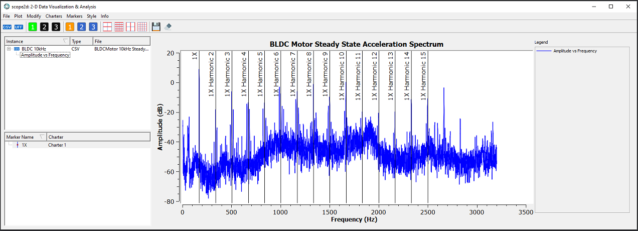
Harmonics and sidebands Top
Vertical markers can have harmonics and sidebands. These are useful specifically in frequency spectrum analysis. Harmonics and sidebands are added to a vertical marker by right clicking the vertical marker on the marker tree and selecting either “Add harmonics” or “Add sidebands”.
Harmonics are defined as vertical markers having X coordinates which are integer multiples of the X coordinate of the fundamental marker (or the first harmonic). For example, say we have a vertical marker at X = 166 Hz for the first shaft order (1X). If we add 14 harmonics to this marker, that means we will have markers at 332 Hz, 498 Hz, 664 Hz etc.
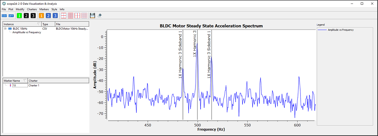
Sidebands are defined as equally spaced neighboring vertical markers which are placed on either sides of the fundamental marker. For example, assume we have a vertical marker at X = 498 Hz. If we add one side band with a gap 15 Hz, we will have a total of two additional markers; one on the left and one on the right, at X values 483 Hz and 513 Hz.
Adding sidebands dynamically Top
In data analysis and especially spectrum (vibration) analysis, sidebands of harmonics may contain important information about the data and the phenomenon its related to. For example, it is known that an amplitude modulation in the time domain data of a signal will appear as sidebands of a specific frequency (modulation frequency) in the signal’s frequency spectrum. And this modulation may be due to a very specific event that is important for the data analyst to know.
To quickly search and identify sidebands in a data, dynamic sideband feature of scope2d may be used. It is similar to the regular way of adding sidebands, which is considered the “static” way since the user needs to enter a specific band gap. On the other hand, in dynamic mode, user selects a “band tick” rather than a band gap and the selections made are instantly updated and shown on the charter. One band tick is equal to a band gap of one times the data step size.
For example, say the X coordinates in the data go like: 0, 0.1, 0.2, 0.3, … Therefore the step size (or resolution) is 0.1. Assume there is a vertical marker at X = 2.0. If the user selects to draw sidebands to this marker with a band tick of 3, then the band gap will be;
Band Gap = Band Tick * Step Size = 3 * 0.1 = 0.3 (in units of the X Axis)
Therefore, the user will see sidebands drawn at 2.0 - 0.3 = 1.7 AND 2.0 + 0.3 = 2.3.
This functionality is designed to identify which data points are actually sidebands of a specific marker in the plot.
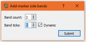
Hint: If you click in the spin boxes for band count and band ticks in dynamic mode, you can use the up and down buttons on the keyboard to quickly increment or decrement the values.
Notes:
-
This functionality is meaningful only when a single curve is analyzed at a time. Therefore, make sure that the charter you are working on has ONLY ONE curve on it when you want to use this functionality.
-
The data MUST be equally spaced along its horizontal (or independent) axis.
Charters Top
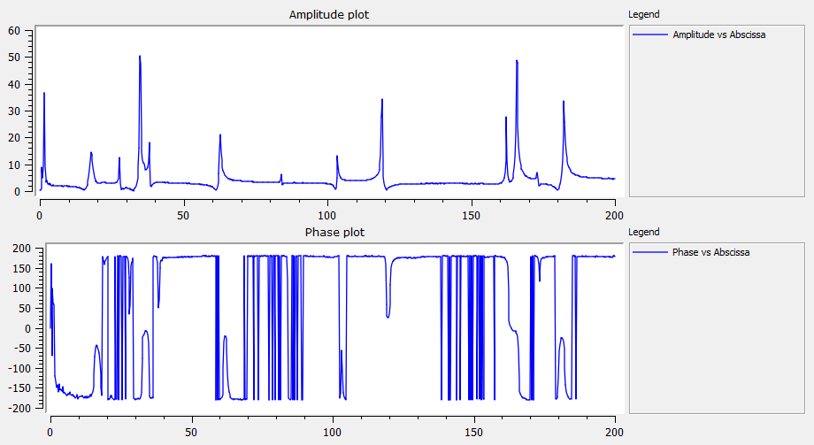
A Charter consists of a canvas to plot on and its legend to show plotted curves. Note that the legend’s width can be adjusted by horizontally dragging it. The legend can be made hidden as well by dragging it to the right until it collapses.
scope2d provides 3 independent charters to be viewed simultaneously. Sometimes it is needed to have multiple charters to view different sets of data which are somehow relevant, for example phase and amplitude plots of a complex signal. In scope2d, it is possible to toggle these 3 charters independently and control them separately by selecting one of them as the active charter. The active charter is the charter that receives the user interactions such as plot commands or style commands.
Toggle charters Top
Use the first set of “1 2 3” buttons to toggle Charter 1, Charter 2 and Charter 3 independently. Green means the charter is shown, black means the charter is hidden.

Active charter Top
You can set one of the charters as the active charters using the second set of “1 2 3” buttons. Orange means the charter is set as the active charter, blue means the charter is not set as the active charter.

Zooming Top
There are two types of zooming in scope2d: Synchronized and Non-synchronized zooming.
-
Non-synchronized zooming: Traditional zooming. press and hold LEFT MOUSE BUTTON on a charter and drag it anywhere to zoom. To revert the last zoom, press MIDDLE MOUSE BUTTON and to revert all zooms, press RIGHT MOUSE BUTTON.
-
Synchronized zooming: When multiple charters are used to analyze multiple sets of relevant data, a synchronized zooming capability between charters is useful. scope2d offers such functionality. When synchronized zoom is used, a unit zoombox will be created first, and then this unit zoombox will be applied to all charters by scaling with respect to axis limits. To sync-zoom multiple charters, while holding down the CTRL key, press and hold LEFT MOUSE BUTTON and drag the cursor anywhere to draw the zoombox.
Plot Scales Top
Different scales can be used to represent the same set of data. There are 4 scales available in scope2d. To select one of the scales available, go to the Plot menu on the top menubar, and then go to Scale. There, you can select one of the 4 scales available. The selected scale will be applied to the active charter only.
Linear scale Top
Both x and y axes are linearly scaled.
Log scale Top
Y axis is logarithmically scaled (base 10). Cannot be applied if the x axis has any negative values.
Log-Log scale Top
Both x and y axes are logarithmically scaled (base 10). Cannot be applied if either the x or the y axis has any negative values.
Normalized scale Top
The selected axis (x or y, or both) can be normalized with respect to a reference value (which cannot be zero). This feature is useful as it can be used for a variety of purposes. An example of such purposes could be obtaining an order-normalized frequency axis for vibration analysis (i.e. frequency axis normalized with respect to shaft rotation speed, or 1X).
When Normalized is selected from the top menubar; firstly, select the axis that you want to normalize:
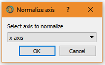
Once the axis is selected, you will be prompted a window to enter the reference value that will be used for normalization. All values on the selected axis will be divided by this value.
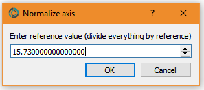
If you want to revert the normalization, simply normalize again with a reference value of 1.0.
Calculators Top
Calculators are a useful feature of scope2d, which allows the user to calculate a dataset’s maximum value, minimum value, mean value, mode and others as well as create a mathematical expression using up to 5 datasets as inputs to calculate a single resulting dataset.
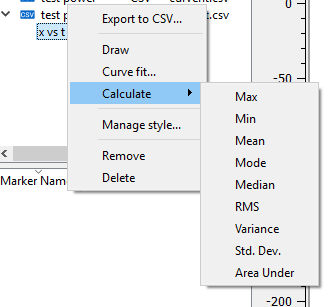
By right clicking a child instance (a plot item on the instance tree) and selecting the “Calculate” menu, it is possible to calculate:
- Maximum value
- Minimum value
- Mean value
- Mode
- Median
- Standard deviation
- RMS (Root Mean Square)
- Area under the curve
for that selected plot curve.
Calculating expressions Top
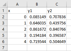
Mathematical expressions such as 1.12 + sin(2*'PI'*'N1') can be calculated using existing datasets as inputs. For example, we have a data that stores the values of X axis as well as the values of the real and imaginary parts of the Y axis. We can use a calculator to calculate the modulus values from the real and imaginary components.
Initially, we begin with below data:
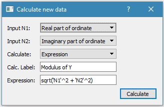
Right click the parent instance of the dataset and select “Calculate”. Set the number of inputs to 2. Select input 1 (N1) as the real part of the Y data and select input 2 (N2) as the imaginary part of the Y data. Make sure that “Calculate” is set to “Expression”. As it is known, modulus is equal to the square root of the summation of the squares of the real and imaginary parts. Therefore, enter sqrt('N1'^2 + 'N2'^2) as the expression and click “Calculate”. This will conduct an element-wise calculation for the elements of N1 and N2.
Calculated datasets are saved as columns in their respective parent instances.

Notes:
- Make sure to apostrophe(‘) right before and after input names. e.g. ‘N1’, ‘N4’ etc.
- All calculation types except for expression are only applicable to a single input. They will produce a new dataset that has equal number of elements as the input, with all values in the dataset being equal to the calculated value.
- In the case of selecting multiple inputs with different lengths, the resulting dataset will have a length equal to the length of the input data with the smallest length.
- When a dataset does not have a mode, the minimum value in the dataset is returned as the mode.
- It is not possible to use datasets from different parent instances as inputs to a calculator.
- The functions supported by the calculators are:
- LOG: Natural logarithm
- LOG10: Base 10 logarithm
- SIN: sine
- COS: cosine
- TAN: tangent
- COT: cotangent
- ASIN: arcsin
- ACOS: arccos
- ATAN: principle value of arctan
- ACOT(x): ATAN(1/x)
- DEG: convert to degrees
- RAD: convert to radians
- SQRT: square root
- EXP: exponential
- ABS: absolute
- Function names can be all uppercase or all lowercase.
- Pi is recognized when entered as ‘pi’ or ‘PI’. e.g. sin(‘pi) or sin(‘PI’)
Curve Fitters Top
Curve fitters give the user the ability for statistical analysis of the data. Available curves are:
- Linear (y = Ax + B)
- Exponential (y = A exp(Bx))
- Logarithmic (y = A lnx + B)
- Power (y = A x^B)
- Polynomial (y = A0 x^0 + A1 x^1 + … + A(n-1) x^(n-1))
- Moving average
Curves are fitted to already-plotted data (child instances). To fit a curve to a child instance, right click that child instance and select “Curve fit”. Curve fitting dialog will pop up; simply select the type of the fit you want to apply and hit “Apply”. The fitted curve will be generated and added as a trendline under the respective child instance. Trendline controls are the same as child instance controls.
To see the fitted curve equation with all its constants in double precision, along with the coefficient of determination (R squared), right click a trendline and select “Curve info”.
scope2d Generic CSV File Format Top
In addition to other supported formats, scope2d has a native generic CSV file format. Any data, taken from any source, can easily be used to create a generic CSV file and scope2d will be able to load it without any issues. Below is an example scope2d generic CSV file, containing 3 data columns, 5 data points for each column and is comma separated.
SCOPE2D_CSV_DATA_START
Example Generic CSV File
x, y1, y2
0.00, 1.12, 5.01
0.10, 2.02, 3.98
0.20, 0.76, 4.11
0.30, 1.65, 1.25
0.40, 0.46, 2.78
SCOPE2D_CSV_DATA_END
As seen in above example file, the file has a total of 9 lines. The start tag in the first line, SCOPE2D_CSV_DATA_START, is the tag scope2d uses to tag the beginning of a data block in a generic CSV file.
The line after the start tag line contains the label or the name of the data block. In this example, the name of the data block is set as Example Generic CSV File.
The third line, which comes after the block name line, contains the data column headers. In this example data, there are 3 data columns which are named x, y1 and y2.
Numerical data begins in the line after the headers line. In every numerical data line, numerical values should be given in appropriate order which respects the order of the headers. Numerical values should use the same delimiter character as the headers. The decimal separator must be a dot and not a comma.
The final line of every data block must contain SCOPE2D_CSV_DATA_END only, which indicates the end of the block.
It is possible to have multiple blocks in the same generic CSV file. For example, one can do:
SCOPE2D_CSV_DATA_START
Measurement 1
x, y1, y2
0.00, 1.12, 5.01
0.10, 2.02, 3.98
0.20, 0.76, 4.11
0.30, 1.65, 1.25
0.40, 0.46, 2.78
SCOPE2D_CSV_DATA_END

SCOPE2D_CSV_DATA_START
Measurement 2
x, y1, y2
0.00, 2.02, 4.21
0.10, 2.82, 1.98
0.20, 0.76, 3.94
0.30, 1.13, 1.25
0.40, 0.12, 2.54
SCOPE2D_CSV_DATA_END
In this example file there are two data blocks, Measurement 1 and Measurement 2.
Therefore, the rules of the format are:
- scope2d generic CSV files can have any file extension
- scope2d generic CSV files can contain multiple data blocks
- For numerical values, decimal separator must be a dot and not a comma
- There must be no empty lines in data blocks
- Data blocks must begin with the tag
SCOPE2D_CSV_DATA_STARTand end withSCOPE2D_CSV_DATA_END - The delimiter should be the same for the headers and the numerical data lines
- After the data start tag, block name should be given
- After the block name line, headers should be given
- After the headers line, numerical data should start
Note: The delimiter can be the whitespace character.
Following these rules, one can easily use any existing data to create a scope2d generic CSV file. Below is an example how.
From Excel to scope2d Generic CSV Top
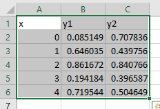
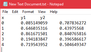
Say we have below data in an Excel file.
To convert this into a generic CSV data, select all cells, including the headers.
Copy the data by hitting CTRL + C. Create a new text file and paste the copied data in the text file.
To convert this data to scope2d generic CSV data, simply add the data start and end lines. Also, the data block name line.
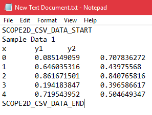
Save the file and close it. Now, this file is a whitespace-delimited scope2d generic CSV file and can be loaded in scope2d using the CSV import option.
Note: This approach works only if the data are listed as columns (i.e. from top to bottom and separated as columns). If the data are listed as rows, such as in the Universal File Format, this approach will not work.